Last updated: 2021-06-18

Checks: 7 0

Knit directory: RainDrop_biodiversity/

This reproducible R Markdown analysis was created with workflowr (version 1.6.2). The Checks tab describes the reproducibility checks that were applied when the results were created. The Past versions tab lists the development history.

R Markdown file: up-to-date

Great! Since the R Markdown file has been committed to the Git repository, you know the exact version of the code that produced these results.

Environment: empty

Great job! The global environment was empty. Objects defined in the global environment can affect the analysis in your R Markdown file in unknown ways. For reproduciblity it’s best to always run the code in an empty environment.

Seed: set.seed(20210406)

The command set.seed(20210406) was run prior to running the code in the R Markdown file. Setting a seed ensures that any results that rely on randomness, e.g. subsampling or permutations, are reproducible.

Session information: recorded

Great job! Recording the operating system, R version, and package versions is critical for reproducibility.

Cache: none

Nice! There were no cached chunks for this analysis, so you can be confident that you successfully produced the results during this run.

File paths: relative

Great job! Using relative paths to the files within your workflowr project makes it easier to run your code on other machines.

Repository version: 31827d3

Great! You are using Git for version control. Tracking code development and connecting the code version to the results is critical for reproducibility.

The results in this page were generated with repository version 31827d3. See the Past versions tab to see a history of the changes made to the R Markdown and HTML files.

Note that you need to be careful to ensure that all relevant files for the analysis have been committed to Git prior to generating the results (you can use wflow_publish or wflow_git_commit). workflowr only checks the R Markdown file, but you know if there are other scripts or data files that it depends on. Below is the status of the Git repository when the results were generated:


Ignored files:
    Ignored:    .Rhistory
    Ignored:    .Rproj.user/
    Ignored:    analysis/site_libs/

Untracked files:
    Untracked:  output/biomass_group_figure.png
    Untracked:  output/richness_figure.png
    Untracked:  output/shannon_figure.png
    Untracked:  output/total_biomass_figure.png

Unstaged changes:
    Deleted:    analysis/about.Rmd

Note that any generated files, e.g. HTML, png, CSS, etc., are not included in this status report because it is ok for generated content to have uncommitted changes.

These are the previous versions of the repository in which changes were made to the R Markdown (analysis/mixed_model_summaries.Rmd) and HTML (docs/mixed_model_summaries.html) files. If you’ve configured a remote Git repository (see ?wflow_git_remote), click on the hyperlinks in the table below to view the files as they were in that past version.

File	Version	Author	Date	Message
Rmd	31827d3	jjackson-eco	2021-06-18	small figure change 2
html	fd1d722	jjackson-eco	2021-06-18	Build site.
Rmd	12fcdf5	jjackson-eco	2021-06-18	small figure change
html	874f8e7	jjackson-eco	2021-06-18	Build site.
Rmd	41af54c	jjackson-eco	2021-06-18	Adding richness + some update to model code
html	dc0db7d	jjackson-eco	2021-06-17	Build site.
Rmd	a40a629	jjackson-eco	2021-06-17	adding other biodiversity measures
html	163466a	jjackson-eco	2021-06-16	Build site.
Rmd	0f76031	jjackson-eco	2021-06-16	Adding to model outputs
html	30cf892	jjackson-eco	2021-06-15	Build site.
Rmd	4c2bd59	jjackson-eco	2021-06-15	mixed model addition + yaml change
html	5b44884	jjackson-eco	2021-06-15	Build site.
Rmd	cbc95ff	jjackson-eco	2021-06-15	wflow_publish(c(“.Rprofile”, “analysis/exploratory_analysis.Rmd”,

Here we present the results of Bayesian hierarchical mixed-effects models to explore how the rainfall treatments have influenced biodiversity, namely, the above-ground biomass (both total at the group level) and species diversity (Shannon-Wiener index and species richness) at the RainDrop site. Please refer to the file code/mixed_effects_models.R for the full details of the model selection. We’ll only be presenting the best predictive models here.

First some housekeeping. We’ll start by loading the necessary packages for exploring the data and the modelling, the raw data itself and then specifying the colour palette for the treatments.

# packages
library(tidyverse)
library(brms)
library(tidybayes)
library(patchwork)
library(gghalves)
library(flextable)
library(vegan)

# load data
load("../../RainDropRobotics/Data/raindrop_biodiversity_2016_2020.RData", 
     verbose = TRUE)

Loading objects:
  biomass
  percent_cover

# wrangling the data
# Converting to total biomass - Here we are considering TRUE 0 observations - need to chat to Andy about this
totbiomass <- biomass %>%
  group_by(year, harvest, block, treatment) %>%
  summarise(tot_biomass = sum(biomass_g),
            log_tot_biomass = log(tot_biomass + 1)) %>%
  ungroup() %>%
  mutate(year_f = as.factor(year),
         year_s = as.numeric(scale(year)))

## group biomass - Focussing on only graminoids, forbs and legumes
biomass_gr <- biomass %>%
  filter(group %in% c("Forbs", "Graminoids", "Legumes")) %>%
  mutate(biomass_log = log(biomass_g + 1),
         year_f = as.factor(year),
         year_s = as.numeric(scale(year)))


# Percent cover - total biodiversity indices
percent_cover <- percent_cover %>%
  drop_na(percent_cover) %>%
  filter(species_level == "Yes")

diversity <- percent_cover %>%
  # first convert percentages to a proportion
  mutate(proportion = percent_cover/100) %>%
  group_by(year, month, block, treatment) %>%
  # diversity indices for each group
  summarise(richness = n(),
            simpsons = sum(proportion^2),
            shannon = -sum(proportion * log(proportion))) %>%
  ungroup() %>%
  mutate(year_f = as.factor(year),
         year_s = as.numeric(scale(year)),
         shannon = as.numeric(scale(shannon)))

# colours
raindrop_colours <- 
  tibble(treatment = c("Ambient", "Control", "Drought", "Irrigated"),
         num = rep(100,4),
         colour = c("#61D94E", "#BFBFBF", "#EB8344", "#6ECCFF"))

Modelling specifications

As seen in the introduction and exploratory analyses, the RainDrop study follows a randomised block design with a nested structure and annual sampling. Each treatment plot occurs within one of 5 spatial blocks, and there is temporal replication across years, and so we used hierarchical models with treatment clustered within spatial block and an intercept only random effect of year (as a factor).

The biodiversity response variables used here are:

Total biomass - \(total\,biomass\) - \(\ln\)-transformed - Gaussian model
Group-level biomass - \(biomass\) - \(\ln\)-transformed - Gaussian model
Shannon-Wiener index - \(shannon\) - z-transformed - Gaussian model
Species richness - \(richness\) - Poisson model with a \(\log\) link

The full base models and priors are given at the beginning of each subsequent section, with the general priors specified for each. Priors were adjusted for each model to prevent divergent transitions, see code/mixed_effects_models.R.

Final models were run over 4 chains, with 4000 iterations of which 2000 were warmup iterations (2000 sampling iterations). We increased the target proposal acceptance probability (i.e. how conservative the acceptance of samples was) of the NUTS sampler by increasing adapt_delta (default = 0.8 from rstan) >= 0.95 (maximum 0.98) in each model to prevent divergent transitions. Model convergence was assessed with \(\hat{R}\).

Model selection

We wanted to assess how the rainfall treatments influenced each of our biodiversity variable, and also how these patterns may have changed through time. We therefore used leave-one-out cross validation implemented in the loo package for a set of candidate models, and assessed differences in estimated out-of-sample predictive performance using model selection. Here, we compared models directly using their expected log pointwise predictive density (elpd). For the full set of models explored for each biodiversity variable, please refer to their specific section.

Generally however, we explored the following additions to the base model:

The rainfall treatment (treatment)
A Linear year effect (year_s)
A functional group effect (group)
An interaction between treatment and year
An interaction between functional group and treatment/year
An interaction between year and harvest point (or collection month)
A year term with temporal autocorrelation (lag 1) (ar(year_s, p = 1))

Autocorrelated year effects

Modelling the temporal component to this dataset alone may not effectively account for temporal autocorrelation in biodiversity, and therefore we implemented autocorrelated year effects with a lag of 1. These autocorrelated terms were implemented using the ar() function of the brms package, in which we specified a lag of 1.

1. Total biomass

The full base model for total biomass is as follows, where for a biomass observation in block \(i\) (\(i = 1..5\)), treatment \(j\) (\(j = 1..4\)) and year \(t\) (\(t = 1..5\))

\[ \begin{aligned} \operatorname{Full model} \\ total\,biomass_{ijt} &\sim \operatorname{Normal}(\mu_{ijt}, \sigma) \\ \mu_{ijt} &= \alpha_{i} + \beta_{harvest[ijt]} + \epsilon_{ij} + \gamma_t \\ \operatorname{Priors} \\ \beta_{harvest[ijt]} &\sim \operatorname{Normal}(0, 1) \\ \alpha_i &\sim \operatorname{Normal}(\bar{\alpha},\sigma_{\alpha}) \\ \epsilon_{ij} &\sim \operatorname{Normal}(0,\sigma_{\epsilon})\\ \gamma_t &\sim \operatorname{Normal}(0,\sigma_{\gamma})\\ \bar{\alpha} &\sim\operatorname{Normal}(3.5, 0.5)\\ \sigma_{\alpha} &\sim \operatorname{Exponential}(3) \\ \sigma_{\epsilon} &\sim \operatorname{Exponential}(3) \\ \sigma_{\gamma} &\sim \operatorname{Exponential}(3) \\ \sigma &\sim \operatorname{Student T}(3,0,2.5) \\ \end{aligned} \]

Where \(\epsilon_{ij}\) and \(\gamma_t\) are intercept-only random effects for the cluster of treatment within block and year, respectively.

Model selection results

load("data/totbiomass_models.RData", verbose = TRUE)

Loading objects:
  totbiomass_treatment
  mod_comp_totbiomass

## model selection table
round(x = mod_comp_totbiomass, 2) %>% 
  rownames_to_column("R object") %>% 
  mutate(`Model terms` = c("treatment", "treatment + year_s",
                           "treatment + year_s + harvest:year_s",
                           "treatment + year_s + treatment:year_s",
                           "base model",
                           "treatment + ar(year_s, p = 1)")) %>% 
  dplyr::select(`R object`, `Model terms`, `LOO elpd` = elpd_loo, 
                `LOO elpd error` = se_elpd_loo, `elpd difference` = elpd_diff,
                `elpd error difference` = se_diff, `LOO information criterion` = looic) %>% 
  flextable(cwidth = 1.5)

R object	Model terms	LOO elpd	LOO elpd error	elpd difference	elpd error difference	LOO information criterion
totbiomass_treatment	treatment	-182.75	12.90	0.00	0.00	365.50
totbiomass_year_linear	treatment + year_s	-182.93	12.89	-0.18	0.33	365.86
totbiomass_year_harvest	treatment + year_s + harvest:year_s	-183.21	12.80	-0.46	0.81	366.42
totbiomass_year_treat	treatment + year_s + treatment:year_s	-183.33	12.61	-0.58	1.96	366.66
totbiomass_base	base model	-187.21	14.37	-4.46	3.91	374.41
totbiomass_year_auto	treatment + ar(year_s, p = 1)	-188.17	11.97	-5.42	5.85	376.34

We can see that the model with the highest predictive performance for total biomass is that with just the treatment effect. There is evidence for a linear year effect and interactions between year and treatment/harvest relative to the base model, but these are not more predictive than just the treatment effect. We have poor support for temporal autocorrelation in the total biomass.

Posterior plots and predictions

First lets have a look at the terms not added after model selection. Here we present distributions from 2000 draws from the posterior of the best model.

totbiomass_treatment %>%
  gather_draws(`b_harvestMid|sd.*|sigma`, regex = TRUE) %>% #tidybayes
  ungroup() %>% 
  ggplot(aes(y = .variable, x = .value)) + 
  stat_halfeye(show.legend = FALSE, fill = "lightsteelblue") +
  scale_y_discrete(labels = c(expression(paste("Early harvest effect ", beta[harvest])),
                              expression(paste("Treatment within block variance ", sigma[epsilon])),
                              expression(paste("Block variance ", sigma[alpha])),
                              expression(paste("Year variance ", sigma[gamma])),
                              expression(paste("Population-level variance ", sigma)))) +
  labs(x = "Posterior estimate", y = NULL) +
  theme_bw(base_size = 20)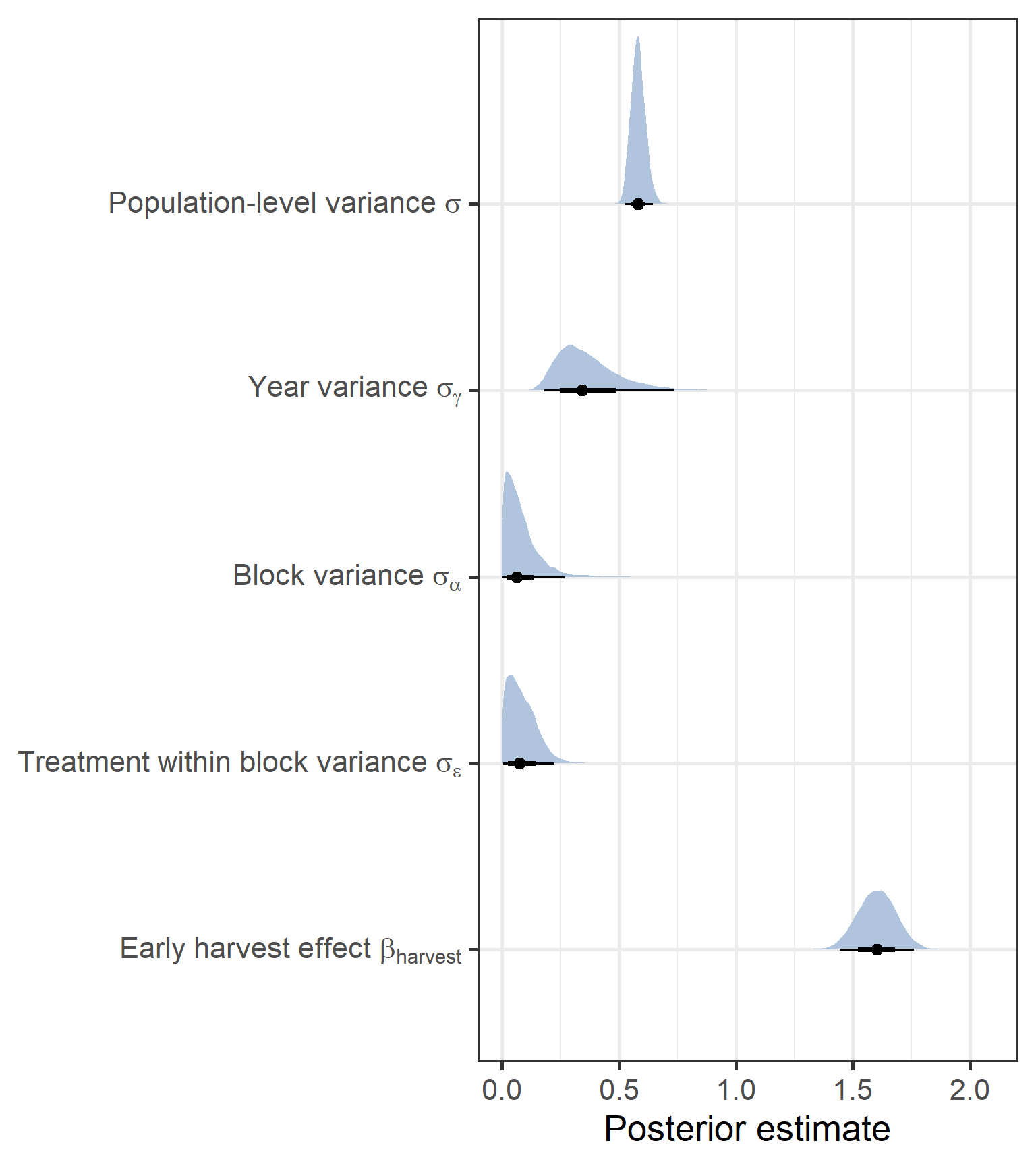

We can see that first of all we have a strong positive effect of the Harvest on total biomass, where biomass is higher by over 50% compared to the later growing season. Then, for the variance terms, we can see that relative to the population-level i.e. total variance, block-level and treatment within block variances were low. In contrast, there was high inter-annual variance.

Now, for the treatment effect. Here we present the mean distribution of posterior predictions for each of the treatment groups and the raw data.

# Harvest labels
harvest.labels <- c("End of season harvest", "Mid season Harvest")
names(harvest.labels) <- c("End", "Mid")

as.data.frame(brms::posterior_predict(totbiomass_treatment)) %>% 
  mutate(sim = 1:8000) %>% 
  pivot_longer(-sim) %>% 
  bind_cols(., slice(totbiomass, rep(1:200, 8000))) %>% 
  mutate(harvest = factor(harvest, levels = c("Mid", "End"))) %>% 
  ggplot(aes(x = treatment, y = value, fill = treatment, group = harvest)) +
  stat_halfeye(width = 0.4, alpha = 0.7) +
  geom_half_point(data = totbiomass, 
                  aes(y = log_tot_biomass, x = treatment, 
                      colour = treatment, group = NULL),
                  side = "l", ## draw jitter on the left
                  range_scale = 0.4, ## control range of jitter
                  alpha = 0.7, size = 2) +
  scale_fill_manual(values = raindrop_colours$colour,
                    guide = F, aesthetics = c("fill", "colour")) +
  labs(x = "Rainfall treatment", y = expression(paste(ln, " Total biomass"))) +
  facet_wrap(~ harvest, ncol = 2,
             labeller = labeller(harvest = harvest.labels),) +
  theme_bw(base_size = 20) +
  theme(panel.grid = element_blank(),
        strip.background = element_blank())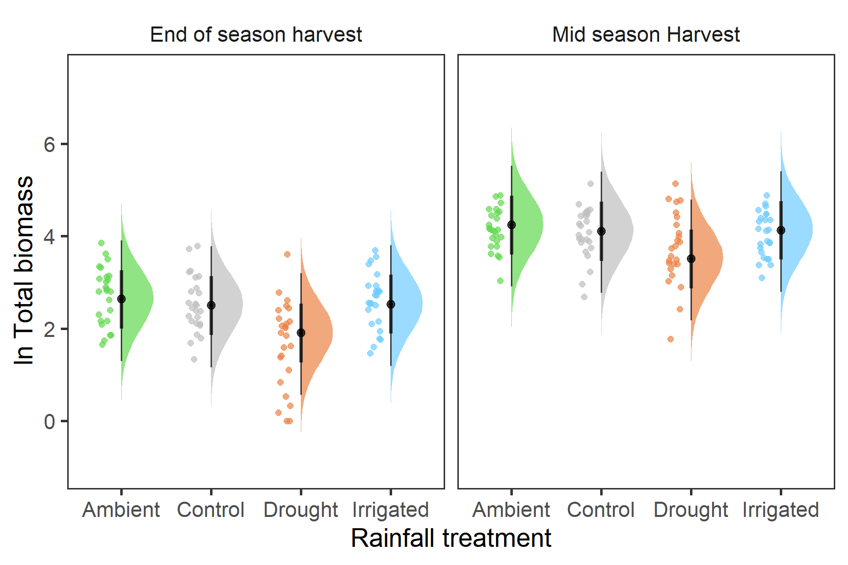

From this it is clear that there is a reduction in total biomass associated with the drought treatment. There doesn’t seem to be any clear differences between ambient, control or irrigated plots however. These differences need to be tested further as well patterns in the variance.

Hypothesis testing

We wanted to test a few key hypotheses

1. What are the ICCs for both the clustered and year random effects

How does the variance in our random effect terms compare to the total variance? An example of this calculation for the block within treatment variance is below

\[ICC_{\sigma_{\epsilon}} = \frac {\sigma^{2}_{\epsilon}}{\sigma^{2}_{\epsilon} + \sigma^{2}_{\alpha} + \sigma^{2}_{\gamma} + \sigma}\] We test the hypothesis of whether this ICC value is equal to zero. First for the treatment within block variance \(\sigma_{\epsilon}\)

h <- paste("sd_block:treatment__Intercept^2/ ", 
           "(sd_block:treatment__Intercept^2 + ",
           "sd_block__Intercept^2 + ",
           "sd_year_f__Intercept^2 + sigma) = 0")

hypothesis(totbiomass_treatment, h, class = NULL)

Hypothesis Tests for class :
                Hypothesis Estimate Est.Error CI.Lower CI.Upper Evid.Ratio
1 (sd_block:treatme... = 0     0.01      0.02        0     0.06         NA
  Post.Prob Star
1        NA    *
---
'CI': 90%-CI for one-sided and 95%-CI for two-sided hypotheses.
'*': For one-sided hypotheses, the posterior probability exceeds 95%;
for two-sided hypotheses, the value tested against lies outside the 95%-CI.
Posterior probabilities of point hypotheses assume equal prior probabilities.

Now the block variance

h <- paste("sd_block__Intercept^2/ ", 
           "(sd_block:treatment__Intercept^2 + ",
           "sd_block__Intercept^2 + ",
           "sd_year_f__Intercept^2 + sigma) = 0")

hypothesis(totbiomass_treatment, h, class = NULL)

Hypothesis Tests for class :
                Hypothesis Estimate Est.Error CI.Lower CI.Upper Evid.Ratio
1 (sd_block__Interc... = 0     0.01      0.03        0     0.09         NA
  Post.Prob Star
1        NA    *
---
'CI': 90%-CI for one-sided and 95%-CI for two-sided hypotheses.
'*': For one-sided hypotheses, the posterior probability exceeds 95%;
for two-sided hypotheses, the value tested against lies outside the 95%-CI.
Posterior probabilities of point hypotheses assume equal prior probabilities.

Finally our inter-annual variance

h <- paste("sd_year_f__Intercept^2/ ", 
           "(sd_block:treatment__Intercept^2 + ",
           "sd_block__Intercept^2 + ",
           "sd_year_f__Intercept^2 + sigma) = 0")

hypothesis(totbiomass_treatment, h, class = NULL)

Hypothesis Tests for class :
                Hypothesis Estimate Est.Error CI.Lower CI.Upper Evid.Ratio
1 (sd_year_f__Inter... = 0     0.19      0.11     0.05     0.48         NA
  Post.Prob Star
1        NA    *
---
'CI': 90%-CI for one-sided and 95%-CI for two-sided hypotheses.
'*': For one-sided hypotheses, the posterior probability exceeds 95%;
for two-sided hypotheses, the value tested against lies outside the 95%-CI.
Posterior probabilities of point hypotheses assume equal prior probabilities.

You can see we have much higher intraclass correlation with the interannual variance, a repeatable year-level biomass, but no clear ICC in our block/treatment effects.

2. Is the difference in biomass between the control treatments is > 0?

Now, we want to test whether the different control plots have a substantially different biomass. Here we are simply testing whether their difference is equal to 0.

hypothesis(totbiomass_treatment, "Intercept - treatmentControl = 0")

Hypothesis Tests for class b:
                Hypothesis Estimate Est.Error CI.Lower CI.Upper Evid.Ratio
1 (Intercept-treatm... = 0     2.79      0.27     2.27     3.34         NA
  Post.Prob Star
1        NA    *
---
'CI': 90%-CI for one-sided and 95%-CI for two-sided hypotheses.
'*': For one-sided hypotheses, the posterior probability exceeds 95%;
for two-sided hypotheses, the value tested against lies outside the 95%-CI.
Posterior probabilities of point hypotheses assume equal prior probabilities.

3. Evidence for an effect of irrigation on biomass relative to ambient?

And finally for any evidence of an irrigation effect

hypothesis(totbiomass_treatment, "Intercept - treatmentIrrigated = 0")

Hypothesis Tests for class b:
                Hypothesis Estimate Est.Error CI.Lower CI.Upper Evid.Ratio
1 (Intercept-treatm... = 0     2.77      0.27     2.24     3.32         NA
  Post.Prob Star
1        NA    *
---
'CI': 90%-CI for one-sided and 95%-CI for two-sided hypotheses.
'*': For one-sided hypotheses, the posterior probability exceeds 95%;
for two-sided hypotheses, the value tested against lies outside the 95%-CI.
Posterior probabilities of point hypotheses assume equal prior probabilities.

2. Group-level biomass

Next we explored the biomass differences between treatments for the three key functional groups: Graminoids, Legumes and Forbs. The full base model here is the same as for total biomass:

\[ \begin{aligned} \operatorname{Full model} \\ biomass_{ijt} &\sim \operatorname{Normal}(\mu_{ijt}, \sigma) \\ \mu_{ijt} &= \alpha_{i} + \beta_{harvest[ijt]} + \epsilon_{ij} + \gamma_t \\ \operatorname{Priors} \\ \beta_{harvest[ijt]} &\sim \operatorname{Normal}(0, 0.5) \\ \alpha_i &\sim \operatorname{Normal}(\bar{\alpha},\sigma_{\alpha}) \\ \epsilon_{ij} &\sim \operatorname{Normal}(0,\sigma_{\epsilon})\\ \gamma_t &\sim \operatorname{Normal}(0,\sigma_{\gamma})\\ \bar{\alpha} &\sim\operatorname{Normal}(1, 1)\\ \sigma_{\alpha} &\sim \operatorname{Exponential}(3) \\ \sigma_{\epsilon} &\sim \operatorname{Exponential}(3) \\ \sigma_{\gamma} &\sim \operatorname{Exponential}(3) \\ \sigma &\sim \operatorname{Student T}(3,0,2.5) \\ \end{aligned} \]

Model selection results

Now we load the results from the model selection and the model with the highest predictive performance and have a look at the results of the model selection. Model terms are additional to those in the base model. For this group-level biomass, we also included terms relating to the functional group (group) of the biomass measure, and appropriate interactions.

load("data/biomass_models.RData", verbose = TRUE)

Loading objects:
  biomass_treatment_group_int
  mod_comp_biomass

## model selection table
round(x = mod_comp_biomass, 2) %>% 
  rownames_to_column("R object") %>% 
  mutate(`Model terms` = c("treatment + group + treatment:group",
                           "treatment + group + year_s + treatment:group + treatment:year_s + group:year_s + treatment:group:year_s",
                           "treatment + group",
                           "group",
                           "treatment",
                           "base model")) %>% 
  dplyr::select(`R object`, `Model terms`, `LOO elpd` = elpd_loo, 
                `LOO elpd error` = se_elpd_loo, `elpd difference` = elpd_diff,
                `elpd error difference` = se_diff, `LOO information criterion` = looic) %>% 
  flextable(cwidth = 1.5)

R object	Model terms	LOO elpd	LOO elpd error	elpd difference	elpd error difference	LOO information criterion
biomass_treatment_group_int	treatment + group + treatment:group	-601.56	17.84	0.00	0.00	1,203.11
biomass_treatment_group_year	treatment + group + year_s + treatment:group + treatment:year_s + group:year_s + treatment:group:year_s	-604.60	17.09	-3.05	3.84	1,209.20
biomass_treatment_group	treatment + group	-629.03	19.01	-27.48	7.75	1,258.07
biomass_group	group	-629.24	18.85	-27.69	8.07	1,258.49
biomass_treatment	treatment	-801.47	15.50	-199.91	14.86	1,602.94
biomass_base	base model	-802.89	15.24	-201.33	15.21	1,605.78

Here the model with the highest predictive performance is the one with a two way interaction between rainfall treatment and functional group. This model has more clear statistical support, with an elpd difference of greater than 3 compared to the second most competitive model.

Posterior plots and predictions

First lets have a look at the terms not added after model selection. Here we present distributions from 2000 draws from the posterior of the best model.

biomass_treatment_group_int %>%
  gather_draws(`b_harvestMid|sd.*|sigma`, regex = TRUE) %>% #tidybayes
  ungroup() %>% 
  ggplot(aes(y = .variable, x = .value)) + 
  stat_halfeye(show.legend = FALSE, fill = "lightsteelblue2") +
  scale_y_discrete(labels = c(expression(paste("Early harvest effect ", beta[harvest])),
                              expression(paste("Treatment within block variance ", sigma[epsilon])),
                              expression(paste("Block variance ", sigma[alpha])),
                              expression(paste("Year variance ", sigma[gamma])),
                              expression(paste("Population-level variance ", sigma)))) +
  labs(x = "Posterior estimate", y = NULL) +
  theme_bw(base_size = 20)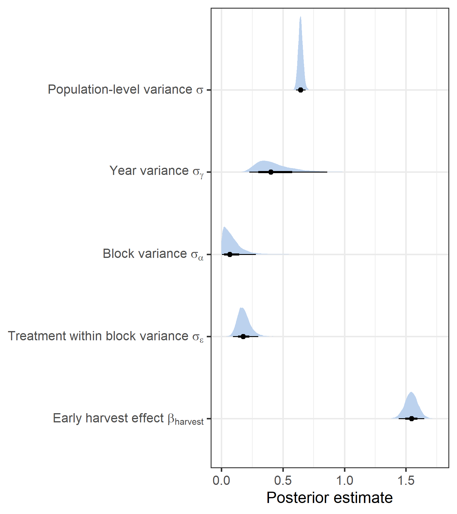

Again we have a strong positive effect of the Harvest on biomass, regardless of functional group, with a similar coefficient. Then, for the variance terms, we see that block/treatment variance terms remain low, but with treatment within block variance slightly higher. Year variance remained high.

Now, for the treatment and group effects. Here we present the mean distribution of posterior predictions for each of the treatment groups and the raw data.

as.data.frame(brms::posterior_predict(biomass_treatment_group_int, nsamples = 2000)) %>% # reducing to make data more manageable 
  mutate(sim = 1:2000) %>% 
  pivot_longer(-sim) %>% 
  bind_cols(., slice(biomass_gr, rep(1:600, 2000))) %>% 
  filter(harvest == "Mid") %>% 
  ggplot(aes(x = treatment, y = value, fill = treatment, group = group)) +
  stat_halfeye(width = 0.4, alpha = 0.7) +
  geom_half_point(data = biomass_gr, 
                  aes(y = biomass_log, x = treatment, 
                      colour = treatment, group = NULL),
                  side = "l", ## draw jitter on the left
                  range_scale = 0.4, ## control range of jitter
                  alpha = 0.7, size = 2) +
  scale_fill_manual(values = raindrop_colours$colour,
                    guide = F, aesthetics = c("fill", "colour")) +
  labs(x = "Rainfall treatment", y = expression(paste(ln, " Total biomass"))) +
  facet_wrap(~ group, ncol = 3) +
  theme_bw(base_size = 20) +
  theme(panel.grid = element_blank(),
        strip.background = element_blank())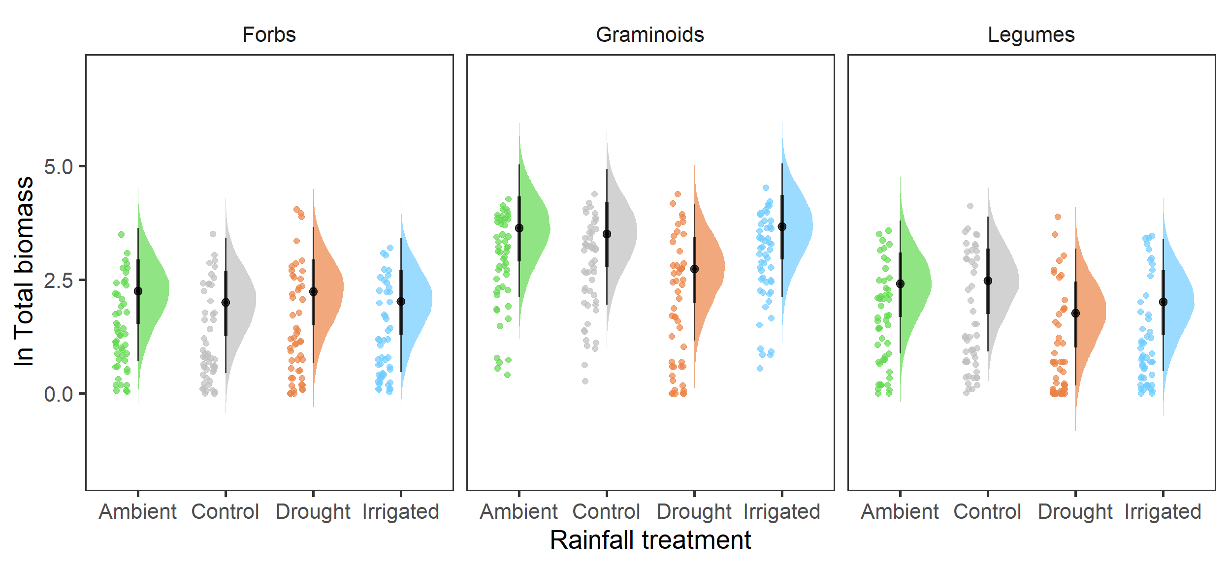

Here we have some very interesting differences in biomass between the functional groups in response to the rainfall treatments. First of all, it is clear that Graminoids are more prevalent than other groups, with \(\beta_{group, graminoid} = 1.39 [1.15,1.64]\). However, we see the negative impact of the drought treatment on biomass is only present in the Graminoids and Legumes, but not the Forbs, which showed little response to the treatments. There is also a slight indication that the Irrigated treatment had reduced Legume biomass \[\beta_{legume:irrigated} = -0.18 [-0.52,0.16]\], but this had weaker statistical support.

Hypothesis testing

1. What are the ICCs for both the clustered and year random effects

Treatment within block variance - slightly higher but still little support

h <- paste("sd_block:treatment__Intercept^2/ ", 
           "(sd_block:treatment__Intercept^2 + ",
           "sd_block__Intercept^2 + ",
           "sd_year_f__Intercept^2 + sigma) = 0")

hypothesis(biomass_treatment_group_int, h, class = NULL)

Hypothesis Tests for class :
                Hypothesis Estimate Est.Error CI.Lower CI.Upper Evid.Ratio
1 (sd_block:treatme... = 0     0.04      0.02     0.01      0.1         NA
  Post.Prob Star
1        NA    *
---
'CI': 90%-CI for one-sided and 95%-CI for two-sided hypotheses.
'*': For one-sided hypotheses, the posterior probability exceeds 95%;
for two-sided hypotheses, the value tested against lies outside the 95%-CI.
Posterior probabilities of point hypotheses assume equal prior probabilities.

Block variance

h <- paste("sd_block__Intercept^2/ ", 
           "(sd_block:treatment__Intercept^2 + ",
           "sd_block__Intercept^2 + ",
           "sd_year_f__Intercept^2 + sigma) = 0")

hypothesis(biomass_treatment_group_int, h, class = NULL)

Hypothesis Tests for class :
                Hypothesis Estimate Est.Error CI.Lower CI.Upper Evid.Ratio
1 (sd_block__Interc... = 0     0.01      0.03        0     0.08         NA
  Post.Prob Star
1        NA    *
---
'CI': 90%-CI for one-sided and 95%-CI for two-sided hypotheses.
'*': For one-sided hypotheses, the posterior probability exceeds 95%;
for two-sided hypotheses, the value tested against lies outside the 95%-CI.
Posterior probabilities of point hypotheses assume equal prior probabilities.

Inter-annual variance - stronger annual variance effect

h <- paste("sd_year_f__Intercept^2/ ", 
           "(sd_block:treatment__Intercept^2 + ",
           "sd_block__Intercept^2 + ",
           "sd_year_f__Intercept^2 + sigma) = 0")

hypothesis(biomass_treatment_group_int, h, class = NULL)

Hypothesis Tests for class :
                Hypothesis Estimate Est.Error CI.Lower CI.Upper Evid.Ratio
1 (sd_year_f__Inter... = 0     0.22      0.12     0.07     0.52         NA
  Post.Prob Star
1        NA    *
---
'CI': 90%-CI for one-sided and 95%-CI for two-sided hypotheses.
'*': For one-sided hypotheses, the posterior probability exceeds 95%;
for two-sided hypotheses, the value tested against lies outside the 95%-CI.
Posterior probabilities of point hypotheses assume equal prior probabilities.

2. Is the difference in biomass between the control treatments is > 0?

hypothesis(biomass_treatment_group_int, "Intercept - treatmentControl = 0")

Hypothesis Tests for class b:
                Hypothesis Estimate Est.Error CI.Lower CI.Upper Evid.Ratio
1 (Intercept-treatm... = 0     0.89      0.34     0.21     1.54         NA
  Post.Prob Star
1        NA    *
---
'CI': 90%-CI for one-sided and 95%-CI for two-sided hypotheses.
'*': For one-sided hypotheses, the posterior probability exceeds 95%;
for two-sided hypotheses, the value tested against lies outside the 95%-CI.
Posterior probabilities of point hypotheses assume equal prior probabilities.

3. Shannon-Weiner diversity index

Now we wanted to get handle on species diversity, starting first with the Shannon-Weiner index. Here we have month instead of harvest (June or September) as it wasn’t a harvest.

\[ \begin{aligned} \operatorname{Full model} \\ shannon_{ijt} &\sim \operatorname{Normal}(\mu_{ijt}, \sigma) \\ \mu_{ijt} &= \alpha_{i} + \beta_{month[ijt]} + \epsilon_{ij} + \gamma_t \\ \operatorname{Priors} \\ \beta_{month[ijt]} &\sim \operatorname{Normal}(0, 1) \\ \alpha_i &\sim \operatorname{Normal}(\bar{\alpha},\sigma_{\alpha}) \\ \epsilon_{ij} &\sim \operatorname{Normal}(0,\sigma_{\epsilon})\\ \gamma_t &\sim \operatorname{Normal}(0,\sigma_{\gamma})\\ \bar{\alpha} &\sim\operatorname{Normal}(3.5, 0.5)\\ \sigma_{\alpha} &\sim \operatorname{Exponential}(3) \\ \sigma_{\epsilon} &\sim \operatorname{Exponential}(3) \\ \sigma_{\gamma} &\sim \operatorname{Exponential}(3) \\ \sigma &\sim \operatorname{Student T}(3,0,2.5) \\ \end{aligned} \]

Model selection results

The model selection took a similar form to previous model selections.

load("data/shannon_models.RData", verbose = TRUE)

Loading objects:
  shannon_treatment_year_int
  mod_comp_shannon

## model selection table
round(x = mod_comp_shannon, 2) %>% 
  rownames_to_column("R object") %>% 
  mutate(`Model terms` = c("treatment + year_s + treatment:year_s",
                           "base model",
                           "treatment + year_s",
                           "treatment",
                           "treatment + ar(year_s, p = 1)")) %>% 
  dplyr::select(`R object`, `Model terms`, `LOO elpd` = elpd_loo, 
                `LOO elpd error` = se_elpd_loo, `elpd difference` = elpd_diff,
                `elpd error difference` = se_diff, `LOO information criterion` = looic) %>% 
  flextable(cwidth = 1.5)

R object	Model terms	LOO elpd	LOO elpd error	elpd difference	elpd error difference	LOO information criterion
shannon_treatment_year_int	treatment + year_s + treatment:year_s	-160.76	8.59	0.00	0.00	321.52
shannon_base	base model	-165.94	9.33	-5.18	3.52	331.88
shannon_year_linear	treatment + year_s	-166.34	9.03	-5.58	3.16	332.68
shannon_treatment	treatment	-166.64	9.18	-5.88	3.49	333.28
shannon_treatment_year_auto	treatment + ar(year_s, p = 1)	-167.58	9.26	-6.82	3.78	335.15

The best model here was the one with an interaction between a linear year effect and the treatment group, the only candidate model better than the base model. This model had strong statistical support however, with an elpd difference greater than 5. Again we found little evidence for an auto-correlated year term.

Posterior plots and predictions

First we present the terms in the base model again.

shannon_treatment_year_int %>%
  gather_draws(`b_monthSept|sd.*|sigma`, regex = TRUE) %>% #tidybayes
  ungroup() %>% 
  ggplot(aes(y = .variable, x = .value)) + 
  stat_halfeye(show.legend = FALSE, fill = "lightsteelblue4") +
  scale_y_discrete(labels = c(expression(paste("September effect ", beta[harvest])),
                              expression(paste("Treatment within block variance ", sigma[epsilon])),
                              expression(paste("Block variance ", sigma[alpha])),
                              expression(paste("Year variance ", sigma[gamma])),
                              expression(paste("Population-level variance ", sigma)))) +
  labs(x = "Posterior estimate", y = NULL) +
  theme_bw(base_size = 20)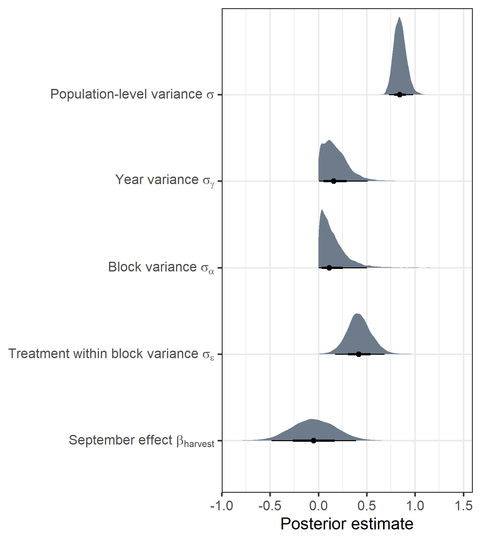

In terms of species diversity, we see some large differences compared to biomass. First, the treatment within block variance was much larger in this measure, suggesting that communities on the site are more localised. There also seems to be less of a variance component for year. Further, There isn’t a clear change in species diversity depending on the observation month.

preddat_shannon <- expand_grid(year_s = seq(-1.15,1.6, length.out = 40),
                               treatment = unique(diversity$treatment),
                               month = "June",
                               block = unique(diversity$block),
                               year_f = unique(diversity$year_f),
                               value = NA) 

shannon_pred <-  brms::posterior_predict(shannon_treatment_year_int,
                                         newdata = preddat_shannon) 

# summary data for each year value
predatsum <- preddat_shannon %>% 
  group_by(year_s, treatment) %>% 
  summarise(value = NA, upr = NA, lwr = NA) %>% 
  ungroup() %>% as.data.frame()
  
for(i in 1:nrow(predatsum)){
  cpos = which(preddat_shannon$year_s == predatsum[i,]$year_s & 
                 preddat_shannon$treatment == predatsum[i,]$treatment)
  
  post_mean = mean(shannon_pred[,cpos])
  cQuant = quantile(shannon_pred[,cpos], c(0.1, 0.90)) # 80% levels
  
  predatsum[i,]$value <- post_mean
  predatsum[i,]$upr <- cQuant[2]
  predatsum[i,]$lwr <- cQuant[1]
  
}

ggplot(predatsum, aes(x = year_s, y = value, group = treatment, 
                      fill = treatment, colour = treatment)) +
  geom_jitter(data = diversity, aes(y = shannon), width = 0.06, size = 2, alpha = 0.85) +
  geom_smooth(stat = "identity", aes(ymax = upr, ymin = lwr), alpha = 0.1) +
  scale_fill_manual(values = raindrop_colours$colour,
                    aesthetics = c("fill", "colour"), name = "Rainfall\ntreatment") +
  labs(x = "Observation year (scaled)", y = "Shannon-Weiner index") +
  theme_bw(base_size = 20) +
  theme(panel.grid = element_blank())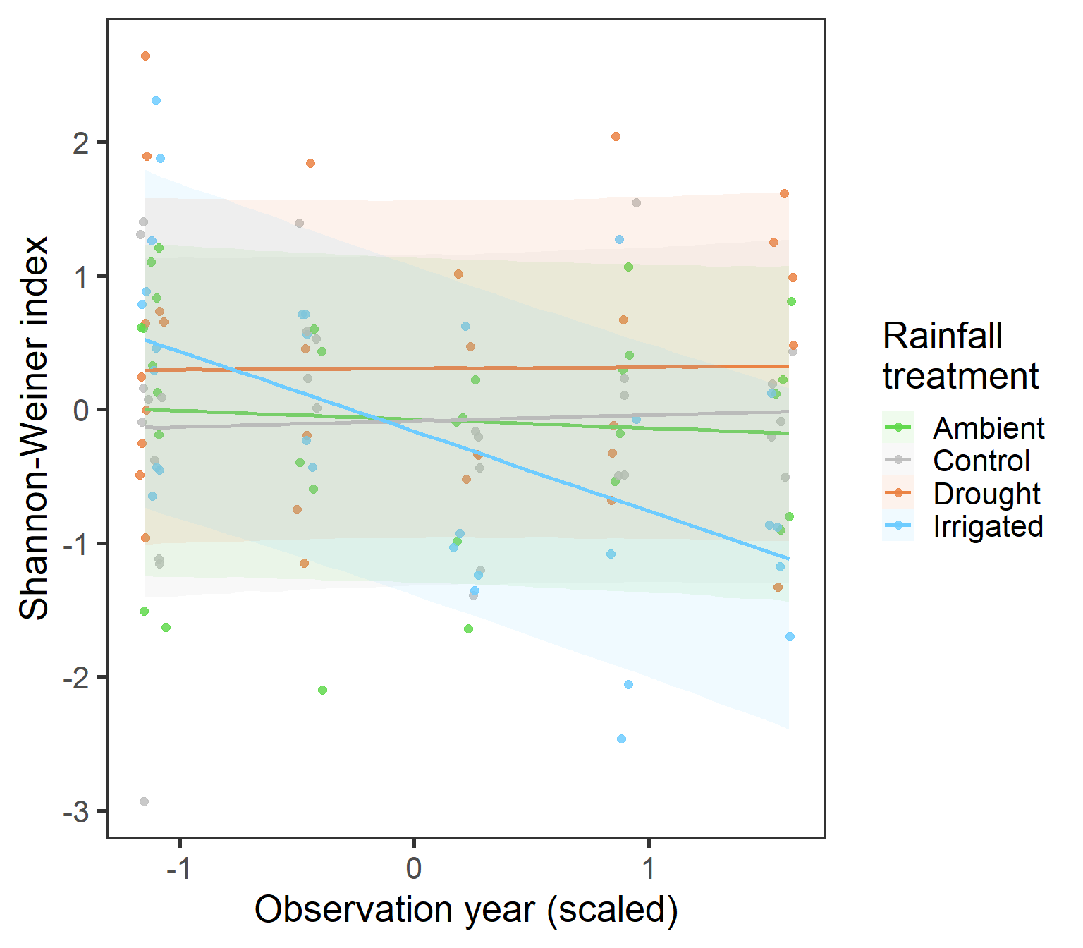

Here, we have a very interesting observation that suggests that as the study has progressed, the Shannon-Weiner diversity in the Irrigated treatments has decreased, but not in other treatment groups. Could this suggest a movement towards an increased monoculture with excessive rainfall?

Hypothesis testing

Here we just want to test the ICC values.

1. What are the ICCs for both the clustered and year random effects

Treatment within block variance - Here this value is the greatest, highlighting the results from before.

h <- paste("sd_block:treatment__Intercept^2/ ", 
           "(sd_block:treatment__Intercept^2 + ",
           "sd_block__Intercept^2 + ",
           "sd_year_f__Intercept^2 + sigma) = 0")

hypothesis(shannon_treatment_year_int, h, class = NULL)

Hypothesis Tests for class :
                Hypothesis Estimate Est.Error CI.Lower CI.Upper Evid.Ratio
1 (sd_block:treatme... = 0     0.17      0.08     0.03     0.34         NA
  Post.Prob Star
1        NA    *
---
'CI': 90%-CI for one-sided and 95%-CI for two-sided hypotheses.
'*': For one-sided hypotheses, the posterior probability exceeds 95%;
for two-sided hypotheses, the value tested against lies outside the 95%-CI.
Posterior probabilities of point hypotheses assume equal prior probabilities.

Block variance

h <- paste("sd_block__Intercept^2/ ", 
           "(sd_block:treatment__Intercept^2 + ",
           "sd_block__Intercept^2 + ",
           "sd_year_f__Intercept^2 + sigma) = 0")

hypothesis(shannon_treatment_year_int, h, class = NULL)

Hypothesis Tests for class :
                Hypothesis Estimate Est.Error CI.Lower CI.Upper Evid.Ratio
1 (sd_block__Interc... = 0     0.03      0.05        0     0.19         NA
  Post.Prob Star
1        NA    *
---
'CI': 90%-CI for one-sided and 95%-CI for two-sided hypotheses.
'*': For one-sided hypotheses, the posterior probability exceeds 95%;
for two-sided hypotheses, the value tested against lies outside the 95%-CI.
Posterior probabilities of point hypotheses assume equal prior probabilities.

Inter-annual variance

h <- paste("sd_year_f__Intercept^2/ ", 
           "(sd_block:treatment__Intercept^2 + ",
           "sd_block__Intercept^2 + ",
           "sd_year_f__Intercept^2 + sigma) = 0")

hypothesis(shannon_treatment_year_int, h, class = NULL)

Hypothesis Tests for class :
                Hypothesis Estimate Est.Error CI.Lower CI.Upper Evid.Ratio
1 (sd_year_f__Inter... = 0     0.04      0.06        0      0.2         NA
  Post.Prob Star
1        NA    *
---
'CI': 90%-CI for one-sided and 95%-CI for two-sided hypotheses.
'*': For one-sided hypotheses, the posterior probability exceeds 95%;
for two-sided hypotheses, the value tested against lies outside the 95%-CI.
Posterior probabilities of point hypotheses assume equal prior probabilities.

4. Species richness

As well as the Shannon-Weiner diversity index, we also wanted to explore patterns in species richness. This variable is count data (no. species) and thus we used a Poisson model with a \(\log\) link

\[ \begin{aligned} \operatorname{Full model} \\ richness_{ijt} &\sim \operatorname{Poisson}(\lambda_{ijt}) \\ \log(\lambda_{ijt}) &= \alpha_{i} + \beta_{month[ijt]} + \epsilon_{ij} + \gamma_t \\ \operatorname{Priors} \\ \beta_{month[ijt]} &\sim \operatorname{Normal}(0, 1) \\ \alpha_i &\sim \operatorname{Normal}(\bar{\alpha},\sigma_{\alpha}) \\ \epsilon_{ij} &\sim \operatorname{Normal}(0,\sigma_{\epsilon})\\ \gamma_t &\sim \operatorname{Normal}(0,\sigma_{\gamma})\\ \bar{\alpha} &\sim\operatorname{Normal}(1, 1)\\ \sigma_{\alpha} &\sim \operatorname{Exponential}(3) \\ \sigma_{\epsilon} &\sim \operatorname{Exponential}(3) \\ \sigma_{\gamma} &\sim \operatorname{Exponential}(3) \\ \end{aligned} \]

Model selection results

The model selection took a similar form to previous model selections.

load("data/richness_models.RData", verbose = TRUE)

Loading objects:
  richness_year_linear
  mod_comp_richness

## model selection table
round(x = mod_comp_richness, 2) %>% 
  rownames_to_column("R object") %>% 
  mutate(`Model terms` = c("treatment + year_s",
                           "treatment",
                           "base model",
                           "treatment + ar(year_s, p = 1)",
                           "treatment + year_s + treatment:year_s")) %>% 
  dplyr::select(`R object`, `Model terms`, `LOO elpd` = elpd_loo, 
                `LOO elpd error` = se_elpd_loo, `elpd difference` = elpd_diff,
                `elpd error difference` = se_diff, `LOO information criterion` = looic) %>% 
  flextable(cwidth = 1.5)

R object	Model terms	LOO elpd	LOO elpd error	elpd difference	elpd error difference	LOO information criterion
richness_year_linear	treatment + year_s	-344.46	5.37	0.00	0.00	688.92
richness_treatment	treatment	-345.44	5.20	-0.98	0.92	690.88
richness_base	base model	-345.48	5.19	-1.02	1.87	690.96
richness_treatment_year_auto	treatment + ar(year_s, p = 1)	-346.22	5.14	-1.76	0.93	692.43
richness_treatment_year_int	treatment + year_s + treatment:year_s	-346.52	5.59	-2.06	0.83	693.04

Here we see the strongest statistical support for the model with year and treatment as univariate effects i.e. excluding interactions. However, this result is less convincing, without a substantial change compared to the base model (difference = 1.02). We conclude that there isn’t a strong impact of treatment on richness, or strong changes through time. However, it is still worth exploring these effects.

Posterior plots and predictions

First again for the base model terms

richness_year_linear %>%
  gather_draws(`b_monthSept|sd.*|sigma`, regex = TRUE) %>% #tidybayes
  ungroup() %>% 
  ggplot(aes(y = .variable, x = .value)) + 
  stat_halfeye(show.legend = FALSE, fill = "paleturquoise4") +
  scale_y_discrete(labels = c(expression(paste("September effect ", beta[harvest])),
                              expression(paste("Treatment within block variance ", sigma[epsilon])),
                              expression(paste("Block variance ", sigma[alpha])),
                              expression(paste("Year variance ", sigma[gamma])))) +
  labs(x = "Posterior estimate", y = NULL) +
  theme_bw(base_size = 20)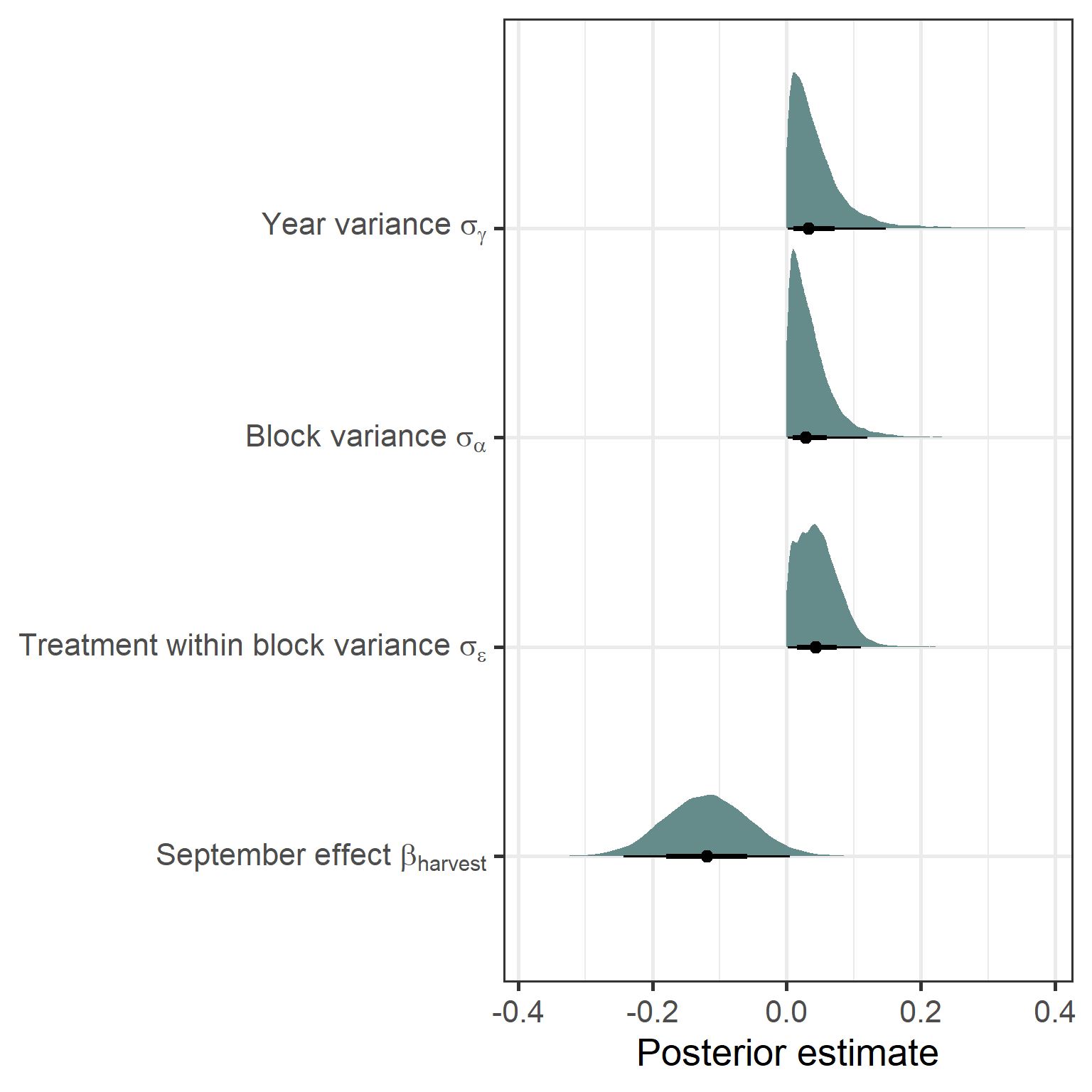

Here we don’t see strong variance effects for any of the random terms. There is a slight negative effect of the late season on richness, but this isn’t that strong.

Now for the treatment and year effects.

# Treatment
p1 <- as.data.frame(brms::posterior_predict(richness_year_linear)) %>% 
  mutate(sim = 1:8000) %>% 
  pivot_longer(-sim) %>% 
  bind_cols(., slice(diversity, rep(1:120, 8000))) %>%
  ggplot(aes(x = treatment, y = value, fill = treatment)) +
  stat_halfeye(width = 0.4, alpha = 0.7) +
  geom_half_point(data = diversity, 
                  aes(y = richness, x = treatment, 
                      colour = treatment, group = NULL),
                  side = "l", range_scale = 0.4, 
                  alpha = 0.7, size = 2) +
  scale_fill_manual(values = raindrop_colours$colour,
                    guide = F, aesthetics = c("fill", "colour")) +
  labs(x = "Rainfall treatment", y = "Species Richness") +
  theme_bw(base_size = 20) +
  theme(panel.grid = element_blank(),
        strip.background = element_blank())

# Year effect
preddat_richness <- expand_grid(year_s = seq(-1.15,1.6, length.out = 40),
                               treatment = unique(diversity$treatment),
                               month = "June",
                               block = unique(diversity$block),
                               year_f = unique(diversity$year_f),
                               value = NA) 

richness_pred <-  brms::posterior_predict(richness_year_linear,
                                         newdata = preddat_richness) 

# summary data for each year value
predatsum <- preddat_richness %>% 
  group_by(year_s) %>% 
  summarise(value = NA, upr = NA, lwr = NA) %>% 
  ungroup() %>% as.data.frame()
  
for(i in 1:nrow(predatsum)){
  cpos = which(preddat_richness$year_s == predatsum[i,]$year_s)
  
  post_mean = mean(richness_pred[,cpos])
  cQuant = quantile(richness_pred[,cpos], c(0.1, 0.90)) # 80% levels
  
  predatsum[i,]$value <- post_mean
  predatsum[i,]$upr <- cQuant[2]
  predatsum[i,]$lwr <- cQuant[1]
  
}

p2 <- ggplot(predatsum, aes(x = year_s, y = value)) +
  geom_jitter(data = diversity, aes(y = richness), width = 0.06, size = 2, alpha = 0.85) +
  geom_smooth(stat = "identity", aes(ymax = upr, ymin = lwr), alpha = 0.1,
              colour = "lightsteelblue4", fill = "lightsteelblue4") +
  labs(x = "Observation year (scaled)", y = "Species richness") +
  theme_bw(base_size = 20) +
  theme(panel.grid = element_blank())

p1 + p2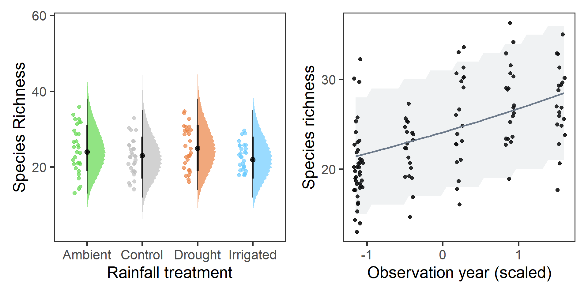

There does look like there was an increase in richness over the study period, although \(\beta_{year} = 0.1 [0.04,0.17]\) and this was not a strong effect (particularly in light of predictive performance in the model selection). However, it does look like on average ~10 more species were observed on the site from 2016-2020. There doesn’t seem to be any strong effect of the treatment groups.

sessionInfo()

R version 4.0.5 (2021-03-31)
Platform: x86_64-w64-mingw32/x64 (64-bit)
Running under: Windows 10 x64 (build 19042)

Matrix products: default

locale:
[1] LC_COLLATE=English_United Kingdom.1252 
[2] LC_CTYPE=English_United Kingdom.1252   
[3] LC_MONETARY=English_United Kingdom.1252
[4] LC_NUMERIC=C                           
[5] LC_TIME=English_United Kingdom.1252    

attached base packages:
[1] stats     graphics  grDevices utils     datasets  methods   base     

other attached packages:
 [1] vegan_2.5-7     lattice_0.20-41 permute_0.9-5   flextable_0.6.5
 [5] gghalves_0.1.1  patchwork_1.1.1 tidybayes_2.3.1 brms_2.15.0    
 [9] Rcpp_1.0.6      forcats_0.5.1   stringr_1.4.0   dplyr_1.0.5    
[13] purrr_0.3.4     readr_1.4.0     tidyr_1.1.3     tibble_3.1.0   
[17] ggplot2_3.3.3   tidyverse_1.3.0 workflowr_1.6.2

loaded via a namespace (and not attached):
  [1] uuid_0.1-4           readxl_1.3.1         backports_1.2.1     
  [4] systemfonts_1.0.1    plyr_1.8.6           igraph_1.2.6        
  [7] splines_4.0.5        svUnit_1.0.3         crosstalk_1.1.1     
 [10] rstantools_2.1.1     inline_0.3.17        digest_0.6.27       
 [13] htmltools_0.5.1.1    rsconnect_0.8.16     fansi_0.4.2         
 [16] magrittr_2.0.1       cluster_2.1.1        modelr_0.1.8        
 [19] RcppParallel_5.0.3   matrixStats_0.58.0   officer_0.3.18      
 [22] xts_0.12.1           prettyunits_1.1.1    colorspace_2.0-0    
 [25] rvest_1.0.0          ggdist_2.4.0         haven_2.3.1         
 [28] xfun_0.22            callr_3.6.0          crayon_1.4.1        
 [31] jsonlite_1.7.2       lme4_1.1-26          zoo_1.8-9           
 [34] glue_1.4.2           gtable_0.3.0         emmeans_1.6.0       
 [37] V8_3.4.0             distributional_0.2.2 pkgbuild_1.2.0      
 [40] rstan_2.21.2         abind_1.4-5          scales_1.1.1        
 [43] mvtnorm_1.1-1        DBI_1.1.1            miniUI_0.1.1.1      
 [46] xtable_1.8-4         stats4_4.0.5         StanHeaders_2.21.0-7
 [49] DT_0.17              htmlwidgets_1.5.3    httr_1.4.2          
 [52] threejs_0.3.3        arrayhelpers_1.1-0   ellipsis_0.3.1      
 [55] farver_2.1.0         pkgconfig_2.0.3      loo_2.4.1           
 [58] sass_0.3.1           dbplyr_2.1.0         utf8_1.2.1          
 [61] labeling_0.4.2       tidyselect_1.1.0     rlang_0.4.10        
 [64] reshape2_1.4.4       later_1.1.0.1        munsell_0.5.0       
 [67] cellranger_1.1.0     tools_4.0.5          cli_2.3.1           
 [70] generics_0.1.0       broom_0.7.5          ggridges_0.5.3      
 [73] evaluate_0.14        fastmap_1.1.0        yaml_2.2.1          
 [76] processx_3.5.0       knitr_1.31           fs_1.5.0            
 [79] zip_2.1.1            nlme_3.1-152         whisker_0.4         
 [82] mime_0.10            projpred_2.0.2       xml2_1.3.2          
 [85] compiler_4.0.5       bayesplot_1.8.0      shinythemes_1.2.0   
 [88] rstudioapi_0.13      gamm4_0.2-6          curl_4.3            
 [91] reprex_2.0.0         statmod_1.4.35       bslib_0.2.4         
 [94] stringi_1.5.3        highr_0.8            ps_1.6.0            
 [97] Brobdingnag_1.2-6    gdtools_0.2.3        Matrix_1.3-2        
[100] nloptr_1.2.2.2       markdown_1.1         shinyjs_2.0.0       
[103] vctrs_0.3.7          pillar_1.5.1         lifecycle_1.0.0     
[106] jquerylib_0.1.3      bridgesampling_1.0-0 estimability_1.3    
[109] data.table_1.14.0    httpuv_1.5.5         R6_2.5.0            
[112] promises_1.2.0.1     gridExtra_2.3        codetools_0.2-18    
[115] boot_1.3-27          colourpicker_1.1.0   MASS_7.3-53.1       
[118] gtools_3.8.2         assertthat_0.2.1     rprojroot_2.0.2     
[121] withr_2.4.1          shinystan_2.5.0      mgcv_1.8-34         
[124] parallel_4.0.5       hms_1.0.0            grid_4.0.5          
[127] coda_0.19-4          minqa_1.2.4          rmarkdown_2.7       
[130] git2r_0.28.0         shiny_1.6.0          lubridate_1.7.10    
[133] base64enc_0.1-3      dygraphs_1.1.1.6

Mixed effects models

Modelling specifications

Model selection

Autocorrelated year effects

1. Total biomass

Model selection results

Posterior plots and predictions

Hypothesis testing

1. What are the ICCs for both the clustered and year random effects

2. Is the difference in biomass between the control treatments is > 0?

3. Evidence for an effect of irrigation on biomass relative to ambient?

2. Group-level biomass

Model selection results

Posterior plots and predictions

Hypothesis testing

1. What are the ICCs for both the clustered and year random effects

2. Is the difference in biomass between the control treatments is > 0?

3. Shannon-Weiner diversity index

Model selection results

Posterior plots and predictions

Hypothesis testing

1. What are the ICCs for both the clustered and year random effects

4. Species richness

Model selection results

Posterior plots and predictions